首先下载wiki的源程序，通过git下载方便随时更新wiki的最新版

git clone https://phabricator.wikimedia.org/source/mediawiki.git

同样wiki的设置需要以下的环境pache + MySQL + PHP，把wiki的源程序软链接到/var/www/html/文件下即在网页中流量。打开网页，根据提示设置各个参数即可。

设置好之后我们得到一个空的wiki百科，没有任何内容，那么下一步就是下载英文wiki百科的备份，并载入这个空的wiki百科中。

下载XML格式的wiki备份，https://dumps.wikimedia.org/enwiki/ , 可以看到最新的wiki整个备份压缩后是17.2GB，解压后大概80GB。

那么下一步就是把解压后的wiki备份文件载入我刚才搭建好的wiki中， 在mediawiki/maintenance/文件夹下运行

sudo php importDump.php –conf ../LocalSettings.php /media/jin/code/wikidata/enwiki-20200701-pages-articles-multistream.xml –username-prefix=””

/media/jin/code/wikidata/enwiki-20200701-pages-articles-multistream.xml 是解压好的wiki备份文件所在的位置

这个过程及其的漫长…………..

结束之后，需要更新wiki百科的网页，运行

php rebuildrecentchanges.php

php initSiteStats.php

最后给出个没有导入完全的wiki测试地址，有效期大约1天。。。

服务器：树莓派 4

操作系统：Raspberry Pi OS

使用树莓派的原因是省电，而且它本身只有卡片大小，携带方便。树莓派的设置非常方便，在没有外接显示器的情况下，我们可以通过ssh链接。初始化的时候，需要在操作系统盘写入空白ssh文件以激活ssh服务。 树莓派系统默认的用户名：pi 密码：raspberry

对于个人网盘的搭建，我选择owncloud, 它本身是开源的，可以在github上下载到源代码，而且对各个平台的支持非常全面，安卓手机，苹果手机，linux，mac等都有客户端支持。

owncloud的设置需要以下的环境Apache + MySQL + PHP

Apache是最常用的网页服务器软件， 在树莓派上安装Apache2，只需要运行

sudo apt install apache2 -y

默认的网页储存在/var/www/html 文件夹下，在浏览器上输入树莓派的ip地址就可以看到这个默认的网页，比如 （http://192.168.1.126）

安装php需要运行

sudo apt install php -y

安装MySQL (MariaDB Server)

sudo apt install mariadb-server php-mysql -y

重启Apache服务

sudo service apache2 restart

下载ownclound源程序并软链接到/var/www/html文件夹下

ln -s /media/usb1/code/owncloud/core owncloud

在浏览器中打开 http://192.168.1.126/owncloud/index.php 进行配置

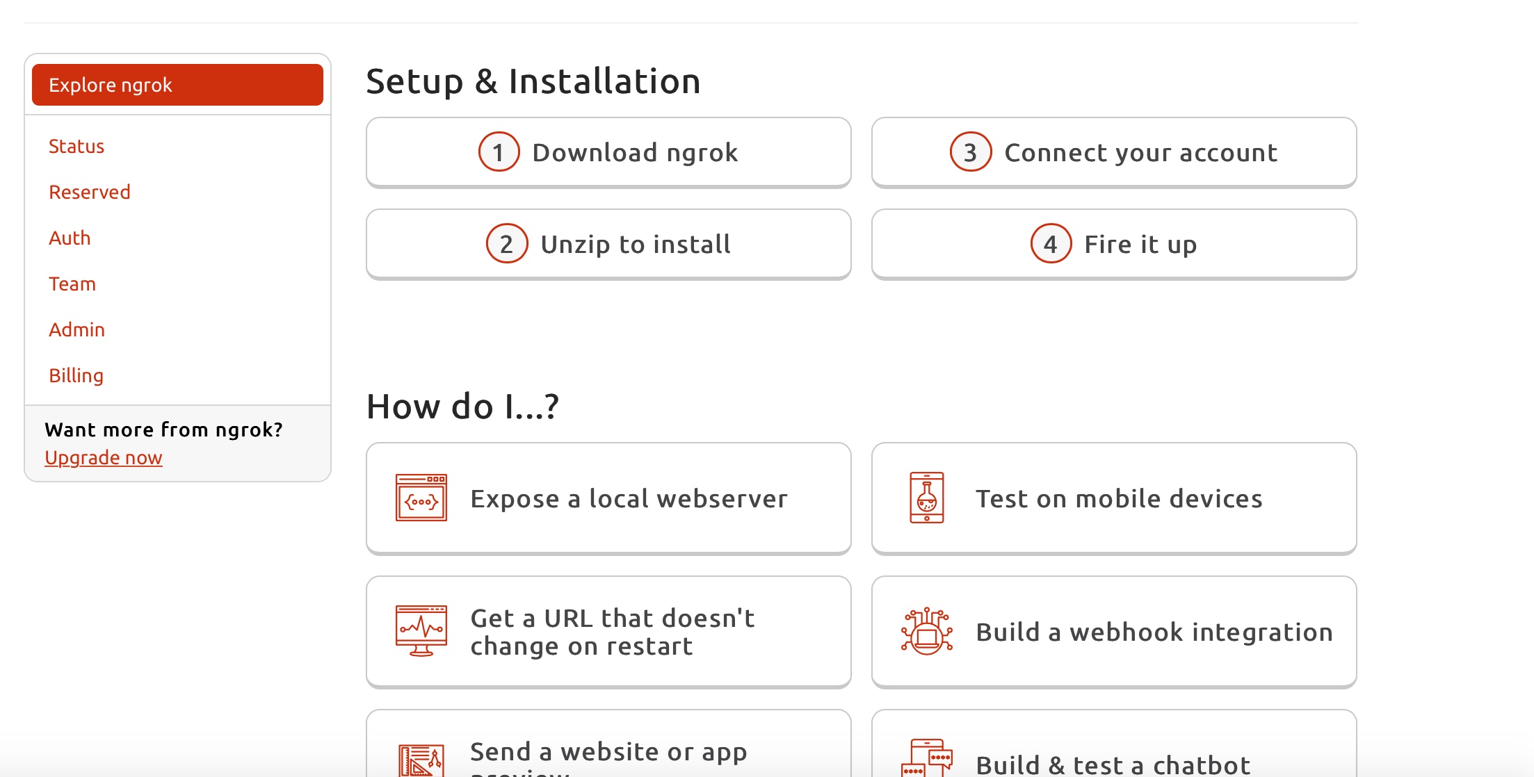
由于我家里的电脑没有公网IP,因此需要进行内网穿透，在这里选取ngrok工具。

免费版本的ngrok没办法后台运行，为了解决这个问题，可以使用screen这个命令

首先安装screen

 apt-get install screen

之后运行

  screen -S 任意名字（例如：keepngork）

然后运行ngrok启动命令

最后按快捷键

 ctrl+A+D

最后贴出一个测试的网址，由于使用的是免费的ngrok,所以不知道链接什么时候会失效，链接在阅读原文可以找到

用户名：test 密码：test

在文章 PHYSICAL REVIEW C 98, 044621 (2018)中，方程被定义为

然而在文章Computer Physics Communications 254, 107340(2020)中，方程被定义为

可以看到上述几个文献中，给出的nonlocal方程在积分项上有分歧。

为了检验上述的几个方程，我们首先来看一下nonlocal potential的单位为何。原则上nonlocal potential应该与local potential的单位一致，对于local potential

它的单位为 MeV fm^{-3}， 也就是说通过积分运算之后nonlocal potential的单位应该与动能的单位一致，即MeV， 也就是说积分项本身要因为的单位为fm^3。 按照这个定义，我们可以排除第一个方程。 对于第二个和第三个方程哪个是正确的，我们先不讨论。 我们先回到R-matrix方法中。对于Lagrange函数的定义

以及

在Pierre最初的文章中，nonlocal potential被定义为

但是，对于Lagrange函数的正交性我们看到这里定义的是一个一维的情况，而并非三维的情况。为了保证三维情况下，径向波函数的正交归一性， Lagrange函数可以被重新定义为

因为对于nonlocal potential项来说

为了验证这个nonlocal项的正确性，我们先把nonlocal potential傅里叶变换到动量空间下求解，对于动量空间下potential是nonlocal，不管坐标空间的potential是local还是nonlocal。因此方便验证坐标空间下的求解是不是正确的，

如上图所示，黑色的线是动量空间下求解的波函数，红色的线是用pierre文章中给出的公式，蓝色的虚线是改正后的nonlocal项。可以看见改正后的项与动量空间下的求解完全一致。

那么现在我们看一下F. PEREY and B. BUCK文章(Nuclear Physics 32 (1962) 353–380)中对nonlocal项的定于与求解为何呢？在其文章中

与Computer Physics Communications 254, 107340(2020)中的定义是一致的，也与改正后的Lagrange-Rmatrix一致

• 第一个工具是linggle， 这是一个在线的平台，可以帮助查找英文短语的搭配。

上图介绍了在linggle搜索短语搭配的几种方式。前段时间一直困惑in addition和in additional两种短语那个正确，多数人和我说没有in additional，于是尝试在上面搜索了一下

结果显示用法还是有的，不过要放在特定的语境里

• 第二个工具是collocaid，这个工具和第一个工作很像，也是找到短语的固定搭配，但是个人感觉这个网站的实用性远远不如上面的那个网站。

• 第三个工具是grammarly， 这是一个在线查找语法错误的平台。强烈推荐这个工具，我经常被合作者抱怨我写的内容有大量的语法错误，有了这个工具的帮助， 我希望能在正确的路上缓慢前行。

• 第四个工具是Manchester Academic Phrasebank。这是一个非常实用的固定搭配数据库，我相信每个需要写论文的人都可以找这个数据库中找到合适的。比如下面的这组用法

Bonaccorso-Brink是一种转移到连续态的反应模型， 它本身是从Hasan和Brink转移到束缚态理论（J. Phys. G 4 (1978) 1573）的一种推广。在转移到束缚态理论中有两个重要的近似。 第一个就是球谐函数的渐进形式，之前已经讨论过了，这种近似的准确度非常的低；第二个就是WKB近似， 也是这里要讨论的内容。

在Brink一系列的半经典理论中的一个出发点就是WKB的分波展开，即Nucl. Phys. A 259 (1976) 99-121这篇文章中的Eq.(3.1)。

那么在这里主要验证一下，这个WKB近似和直接求解薛定谔方程有何区别， 这里我们主要考虑连续态波函数的情况。 首先我们考虑势能为零的情况，量子理论中我们知道这个是平面波的情况。Eq.(3.1) 变为

但是在量子理论中我们知道s-wave的平面波为spherical Bessel function

可以看到中间差了1/4 pi这个系数

那么现在考虑只有p-wave的平面波，通过数值求解我们得到下面的结果

可以看到WKB近似与精确解相比有一个微小的相移(phase shift)。老板跟我说在半经典理论中，centrifugal barrier通常取以下的近似值(文献来源尚无考证)

把这个新的centrifugal barrier代入WKB计算，可以得到

可以看到除了经典的拐点之外，WKB的近似结果还是比较令人满意的。在测试中我测试过l=40的情况，结论是一致的,WKB是一个比较成功的近视。

那么下面我们做进一步的测试， 如果只加入库伦相互作用力会是什么样，我们假设z1=1, z2=1, Elab=160 MeV。数值计算结果如下

可以看到在这里我们的结论基本与平面波一致，即除了s-wave以外的分波WKB与精确解基本一致。同样我们也测试到了l=40的情况。

那么接下来，我们测试一下一个real absorption势的情况，定义这个势具有以下的参数

&POTENTIAL ptype=1 a1=0 a2=208 rc=1.3 uv=77.3 av=0.77 rv=1.15 /

数值计算结果如下

在这里，我们可以得到两个信息，

（1） WKB解与精确解在波函数幅度上存在一定的差别，这个差别除了s-wave之外是一致的；

（2）在小分波的时候，WKB与精确解的phase是一致的，但是当分波变大的时候明显存在相移，而且相移随着分波越大越明显。

上面的第一点可以从Nucl. Phys. A 259 (1976) 99-121的原文中得到解释，在Eq(2.6)中他们假设

然而实际情况并非如此，波函数只是正比于上述的表达式。 那么第(2)条，我们如何来解释呢？

在和老板聊了之后发现，造成这样的原因就是势阱深度数值太大，uv=77.3 MeV，这个数值与Elab=160 MeV相差不多， 所以WKB在这里失效。。然并卵，按照这个逻辑， 那么WKB就不能应用到核反应才对， 因为大多数的情况势阱深度数值都很大！ 这个根本就说不通

今天花了点时间看了一下，她的这篇文章。 这篇文章主要的内容是她把她和她博士导师发展那套半经典散射模型应用到了晕核参与的核反应中。在半经典模型，即eikonal模型中，散射的相移因子和光学势的虚部直接相关。 通过研究相移因子在核反应中的变化从而研究散射过程中截面和光学势虚部的依赖关系。

在这篇文章中， 她假设晕核核反应的光学势虚部由两部分组成，即体项（Volume）和表面项（surface）。这个附加的表面项体现了晕核束缚态波函数在坐标空间下长程的性质。通过她的模型分析，最终得到的结论是表面项的弥散度与晕核的束缚能直接相关,即

把上述公式代入晕核11Be参与的核反应中，我们得到

这个数值在误差范围内完全与后面PRL文章中的结果一致。

对于(+) state，

对于(-)* state

使用关系式 ， 上式变为

使用关系式， 可以得到

对于具有下面形式的inhomogeneous方程

通常情况下有两种解法，一个是微分解法，另外一种是积分解法。对于微分解法来说，我们一般假设

因此上述方程在分波表述下， 可以写为

上面的这个方程可以用Numerov或者R-matrix方法来解。

另外一方面我们还可以通过积分方程来解inhomogeneous equation，

根据定义我们可以得到下列方程

主要注意的是在实际物理应用时，我们通常情况下得到的是完整的source项，即S项，需要通过除以r变成\rho项。

最开始的时候在自己手上的macbook pro上做模型训练，发现速度真的跟蜗牛爬差不多。因此本着白嫖的心态，在网上搜索免费的GPU资源。发现Google旗下的colab可以获得免费强大的Tesla K80单片，如果每个月交9.9美元的话就可以获得更强大的Tesla P100。

但是问题是colab支持的是jupyter nootbooks格式，如果想在colab上做模型训练必须要把faceswap代码转换成jupyter nootbooks吗？难道不可以使用ssh直接连接colab吗？继续搜索发现以下解决方案：

• 首先借助Ngrok，它是一个连接公共网络和本地网络的一个代理软件，需要在它的网站上注册一个账号，并且下载运行它的软件，让这个网站可以通过特定的识别码找到你的本地电脑。当然它也是免费的

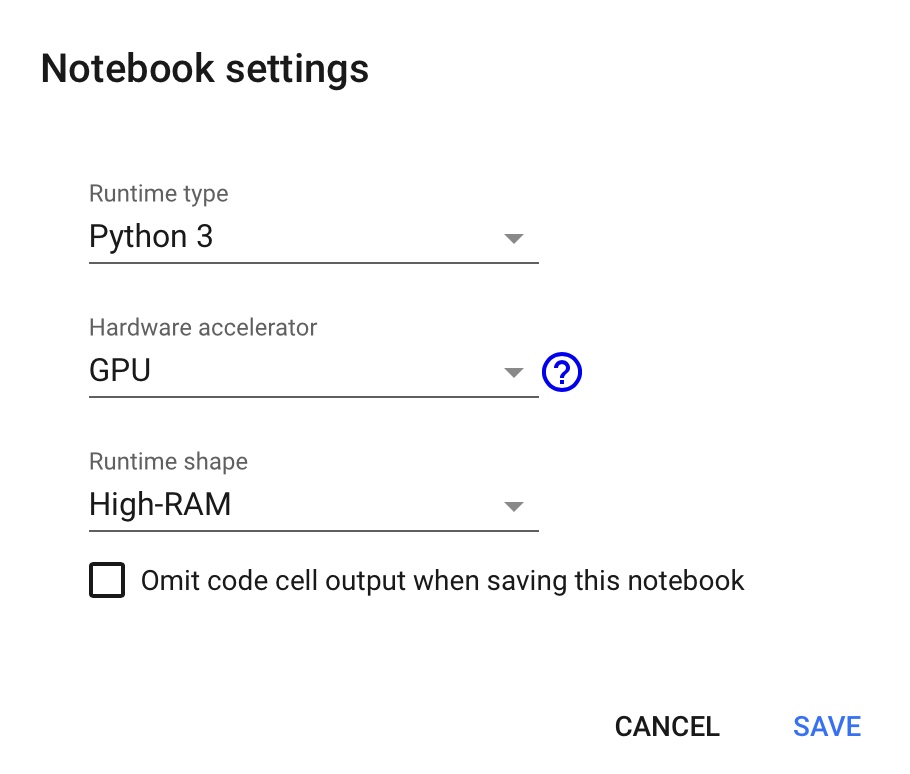
• 建立一个新的colab notebook， 点开Edit->Notebook settings,选中GPU和python3

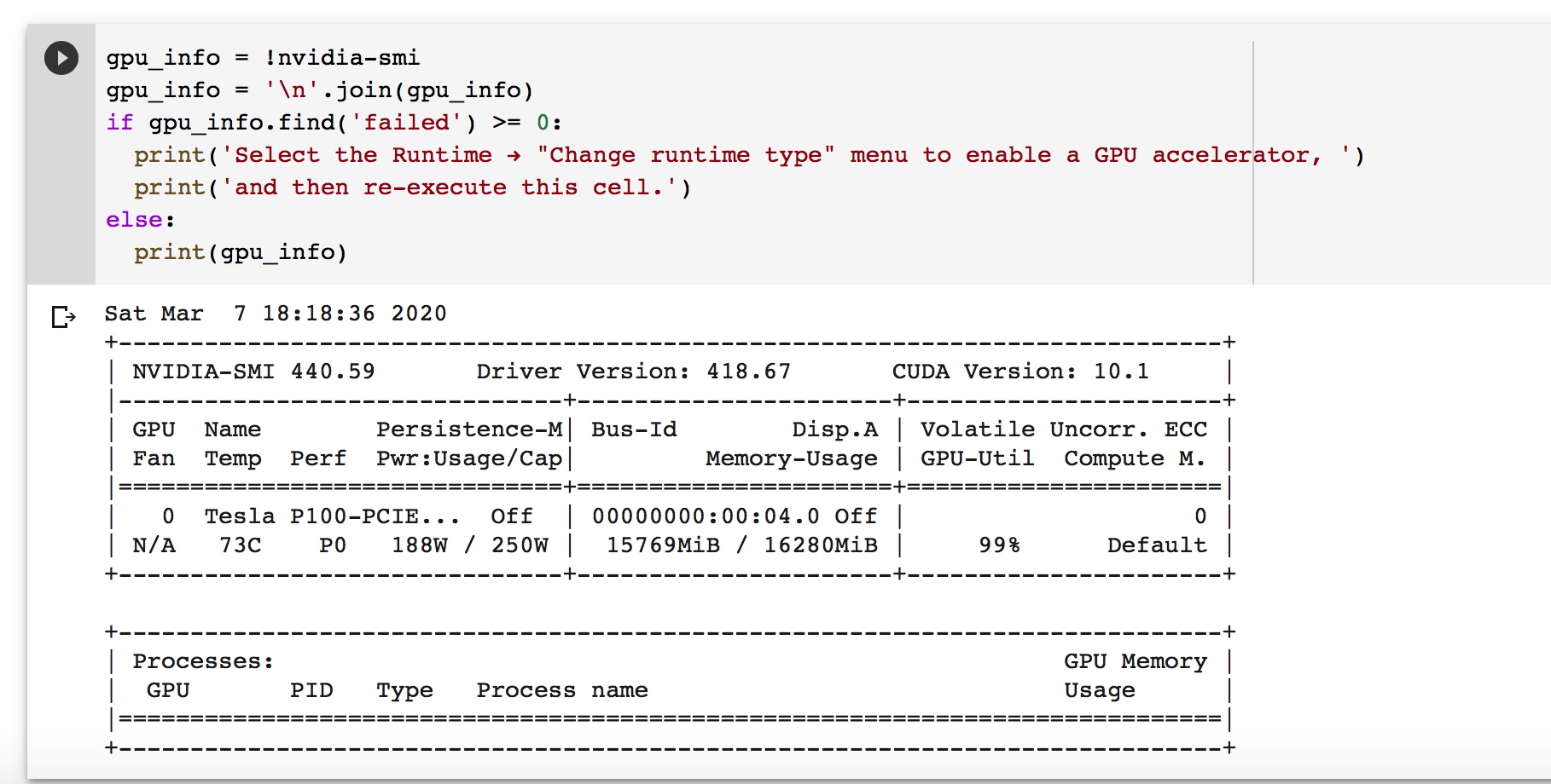
• 复制运行以下代码显示分配到的GPU信息，如下所示我分配到了16G显存的P100

  gpu_info = !nvidia-smi
  gpu_info = ‘\n’.join(gpu_info)
  if gpu_info.find(‘failed’) >= 0:
  print(‘Select the Runtime → “Change runtime type” menu to enable a GPU accelerator, ‘)
  print(‘and then re-execute this cell.’)
  else:
  print(gpu_info)

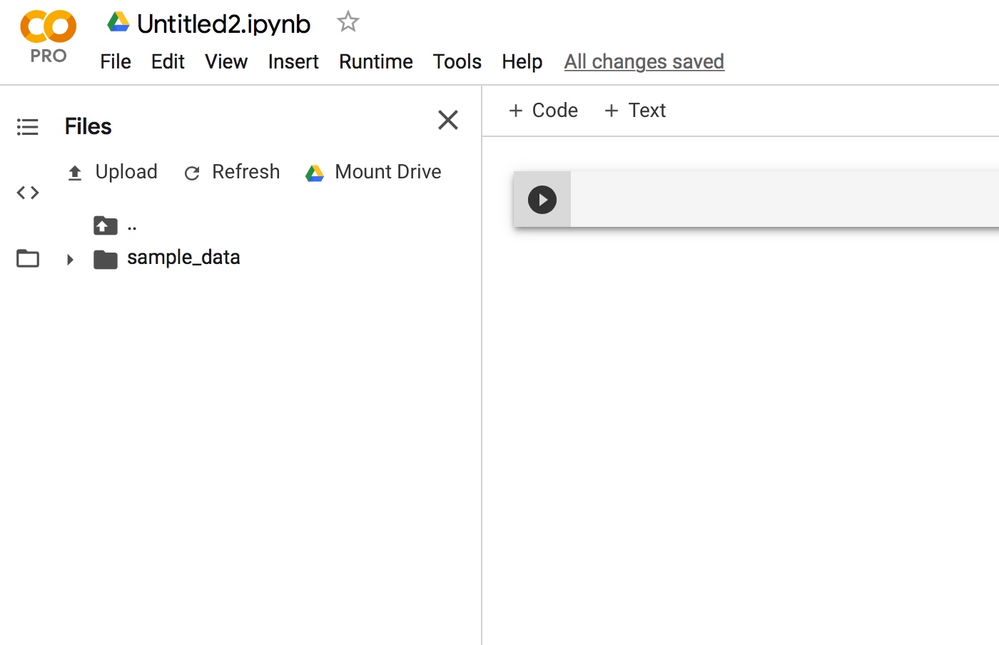
• 挂载Google drive

• 复制运行以下代码。根据提示输入相关的信息，建立ssh代理通道

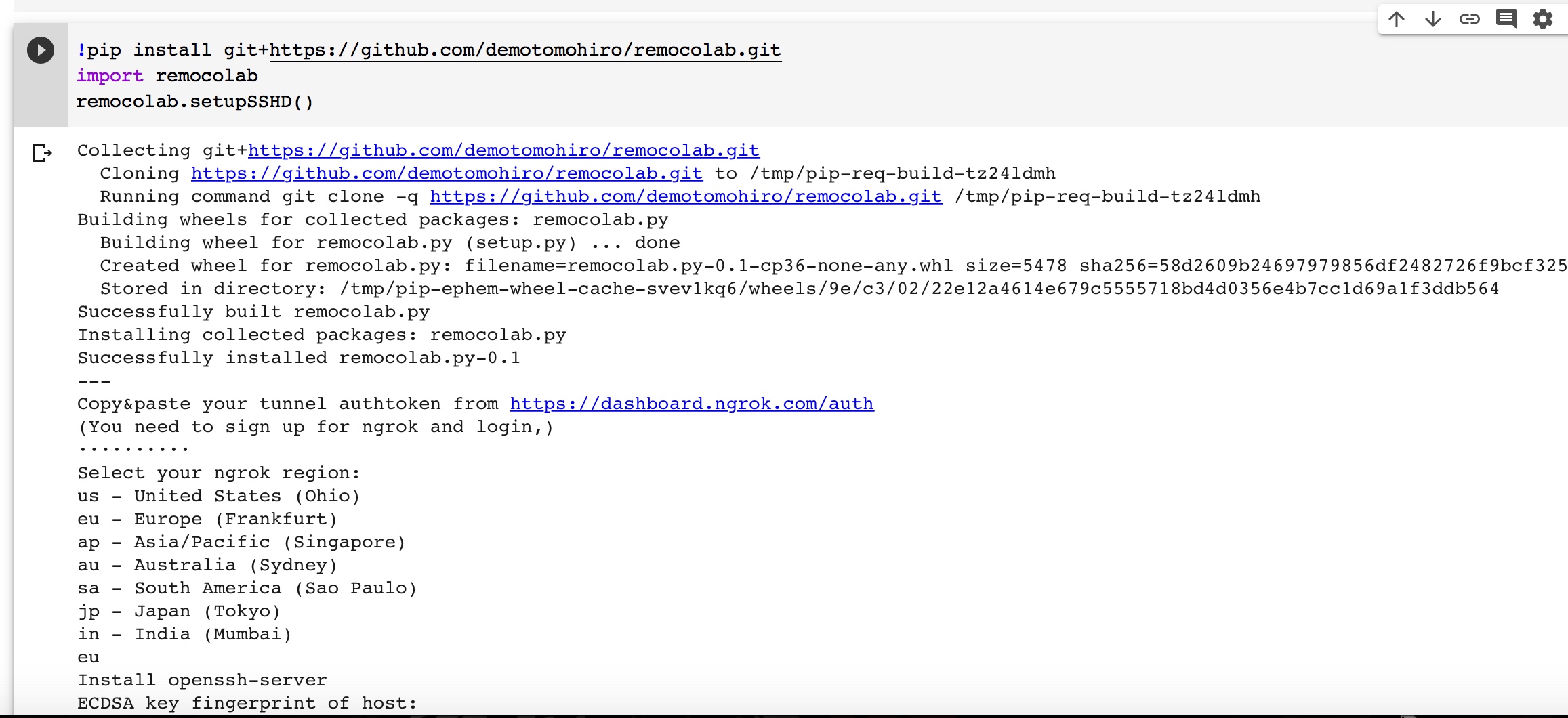
!pip install git+https://github.com/demotomohiro/remocolab.git
import remocolab
remocolab.setupSSHD()

• 根据输出的提示即可使用ssh连接到服务器

• 因为colab分配的服务器，会不定时的刷新重启，因此没有办法在colab本地云盘储存东西，需要通过Google drive挂载，这样其实更加方便使用。 ssh连接到服务器后需要获得超级管理员身份才能进去Google drive的目录，超级管理员密码在上一步有显示，只需输入su, 然后进入Google drive目录/content/drive/My\ Drive/

接下来就是使用faceswap进行换脸的实际操作部分了：

• git clone faceswap的源代码

git clone https://github.com/deepfakes/faceswap.git

• 挂载显卡驱动

  export LD_PRELOAD=/usr/lib64-nvidia/libnvidia-ml.so

• 安装faceswap

  python3 setup.py

  • 选择N,N,Y,Y

• 准备好需要换脸的两个人的照片+视频。 运行下面代码可以从视频中提取人脸

  python3 faceswap.py extract -i source/yifei/videoplayback.mp4 -o source/yifei/face -D s3fd -A fan -M extended -nm hist -min 20 -l 0.4 -een 1 -sz 256 -si 0 -L INFO

  • -i 后面接的是要提取的视频，
  • -o后面是提取的脸存储的目录
  • 这步骤会产生一个videoplayback_alignments.fsa，这个文件储存的是对应视频中人脸的位置，在最后给视频换脸的时候程序需要这个文件来找到视频中需要换的人脸。

• 在提取人脸的时候，程序可能会把不是人脸的东西识别成人脸，因此需要手动将这些删除，faceswap提供了以下的工具，可以将相似的图片排列起来，然后把不是想要换的人脸删除即可

  python3 tools.py sort -i source/yifei/face -s face -t -1.0 -fp rename -g hist -b 5 -be GPU -lf sort_log.json -L INFO

  • -i后面是要排列图片所在的文件夹

• 在删除不必要的图片后，要运行以下代码更新.fsa文件

  python3 tools.py alignments -j remove-faces -a source/yifei/videoplayback_alignments.fsa -fc source/yifei/face -o console -een 1 -sz 256 -L INFO

  • -a 后面接的是fsa文件，
  • -fc后面接的是人脸文件夹

• 在准备好需要换脸的两个文件夹后，就可以进行模型训练了， 运行以下代码

python3 faceswap.py train -A source/yifei/face -ala source/yifei/videoplayback_alignments.fsa -B faces/ofelia -m model/yifei -t Villain -bs 32 -it 1000000 -s 100 -ss 25000 -tia source/yifei/face -tib faces/ofelia -to output/yifei -ps 50 -L INFO

• 值得注意的是，这个命令是要把B的脸换到A上的训练
• -A 后面接的是A脸的文件夹
• -B 后面接的是B脸的文件夹
• -m 后面接的是训练的模型储存的位置
• -t 后面接的是训练的方法，官网上给出了好几种模型训练方法，从基础的Lightweight到最佳的Villain， 根据我在Tesla P100显卡的实际测试来看，这几个模型的训练时间相差不大，因此可以选择最佳的Villain
• -tia 后面接的是想要查看换脸效果的A脸所在的文件夹
• -tib 后面接的是想要查看换脸效果的B脸所在的文件夹
• -to 后面接的是实时输出换脸效果的照片的文件夹，基本上每隔5分钟，会产生一个对比照片。
• -bs 即Batch Size， 每次训练读取脸的数目
• -it 要进行训练的最大次数
• -s 每XX次训练储存一次模型
• -ss 每XX次训练备份一次模型

• 当实时输出换脸效果的照片基本满意的时候，就可以对整个视频进行换脸了

  python3 faceswap.py convert -i source/yifei/videoplayback.mp4 -o output -al source/yifei/videoplayback_alignments.fsa -m model/yifei -c color-transfer -M extended -sc none -w ffmpeg -osc 100 -l 0.4 -j 0 -k -L INFO

  • -i 后面接的是换脸的视频
  • -o 后面接的是换脸结果存放的位置
  • -al 后面接的是.fsa文件，即存储的视频中需要换的脸在视频中位置
  • -m 后面接的是换脸模型的位置

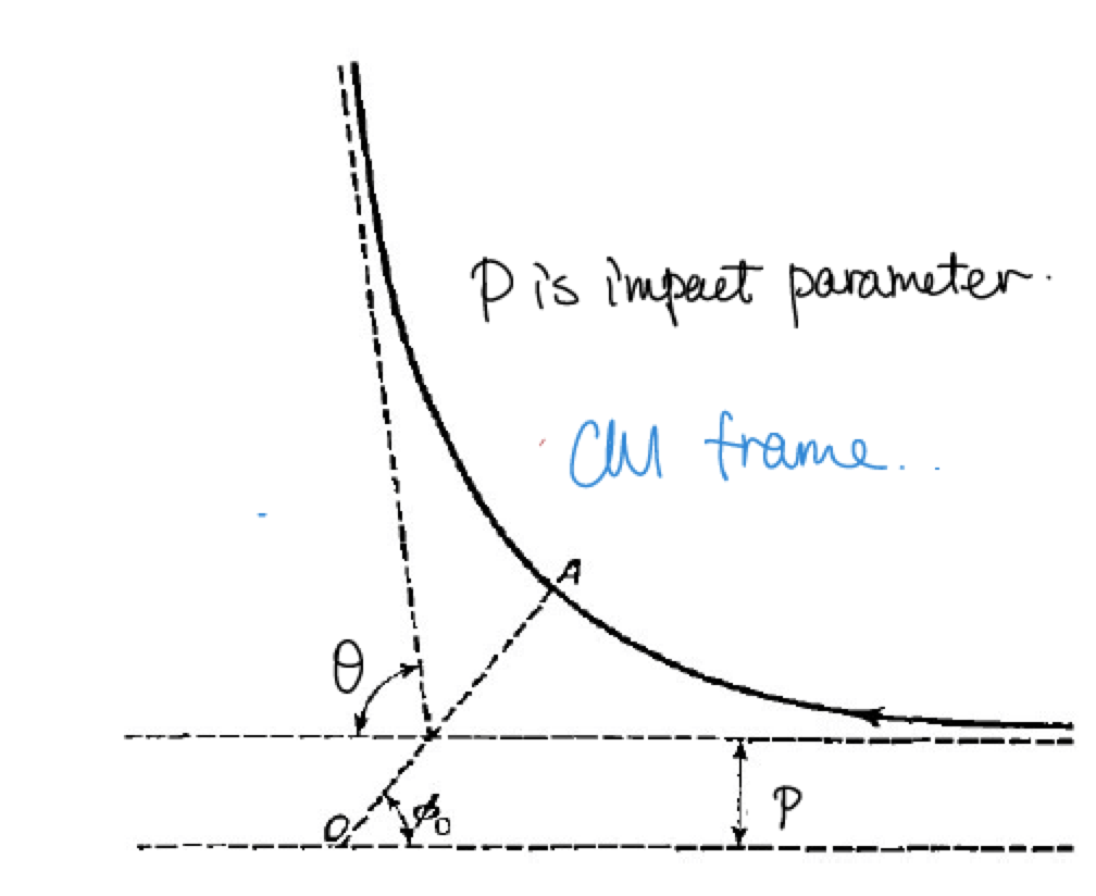
我们考虑一个简单的二维平面内的散射问题。 在质心系下，假设入射粒子流以相同的速度v_in入射。不同的入射粒子通常具有不同的碰撞参数，因此有不同的散射角度\theta。定义dN为单位时间内通过角度区间\theta到\theta+d\theta范围内的粒子数目。这个数目本身并不能很好的描述散射过程，因为它与入射粒子流的密度成正比。 因此我们采用它们之间的比值

其中n是单位时间内通过单位面积的粒子数。 可以发现，这个比值具有面积的量纲，通常把它称为截面

接下来我们讨论一下入射粒子的轨迹, 如上图所示，在中心力场下的散射轨迹以入射粒子到散射中心最短距离（OA）为中心线对称的。两条轨迹渐近线与中心对称线的夹角（\phi_0）是相同的。因此散射角\theta等于

另外，入射粒子的散射问题，可以看成是在中心力场U(r)下的散射，在质心系下总能量为

其中角动量P_L被定义为

因此，我们得到入射粒子的速度为

通过角动量的定义，我们可以得到

接下来我们把入射粒子速度定义中的dt代入上式中，可以得到

其中r_{min}为入射粒子与靶核的最短距离，也是上式根号内表达式为0时的r值。为了方便后续的讨论，我们使用入射粒子速度v_in和碰撞参数p为变量，入射粒子能量与角动量可以表述为

因此\phi角的公式可以改写为

通过\phi角与\theta角的关系式，我们得到碰撞参数与散射角的关系式。 通过上述表达式可以发现，一个\phi角只对应一个碰撞参数。 因此当碰撞参数处于p(\theta)和p(\theta)+dp(\theta)之间时，散射角度对应的区间为\theta到\theta+d\theta。通过该散射角区域的粒子数可以由半径为p和p+dp之间环形的面积乘以粒子流密度n求得，

因此我们可以得到散射截面为

为了找到散射截面与角度的关系， 上式可以改写成

在三维空间下，我们可以对坐标进行球坐标展开，并假设散射对于phi角是各向同性的，我们通常用立体角代替上式的\theta角，

另外对于库伦散射，我们只需要把上面讨论的相互作用势U设为库伦势即可。

经典散射轨迹

我们假设散射发生在二维平面内， 那么经典散射轨迹可以通过求解下式获得